Binary Search Algorithm with Examples

In this post we will discuss one of the most famous algorithms – Binary Search Algorithm with Examples. It may look deceptively simple but it is extremely powerful nonetheless. What makes Binary Search better than Linear Search? How are its Time and Space complexities calculated? All such questions will be answered along with some interesting examples to get an actual feel of the algorithm. So without further ado, let’s begin!

Why Binary Search?

The best way to answer this question is through a very classic problem –

Problem Statement: Given a sorted array of integers, find if target element 10 exists in the array.

Brute Force Method

You wanna find something? Then iterate over all the integers in the array one by one and see if any of them equals 10. Simplest logic ever!

Well, we have a name for this algorithm – Linear Search.

Time Complexity: O(N), N = size of array

Space Complexity: O(1), constant space.

Okay, that’s good. But can we do better? Are we utilizing the fact that the array is sorted? Not really…

And that’s how Binary Search comes into picture.

Binary Search Method

The main idea is to break the array into two equal parts and compare the target with the middle element.

If the target < middle element, search in the left part.

If the target == middle element, return True.

If the target > middle element, search in the right part.

Let’s have a look at the code below.

Let’s dry run our code for the given problem. Our target is to find target = 10 in the sorted array.

Step 0: Just an initial step listing down the input variables.

arr : [-5,0,1,5,7,8,10,50,90,100], target : 10

Step 1: Time to break arr in half, mid = 7.

Left Half: [-5,0,1,5], Right Half: [8,10,50,90,100]

As 10>7, we go towards the right of mid.

Step 2: mid = 50. Again we have two parts –

Left Half: [8,10], Right Half: [90,100].

As 10<50, go to Left.

Step 3: mid = 8. Two parts are –

Left Half: [], Right Half: [10].

Obviously we go Right.

Step 4: mid = 10. Hurray! We reached our target, so return True.

So it took us just 4 steps to reach our target, much lesser than what we’d have required if we went linear!

Time Complexity

At every step, we are reducing the search space by half! This means, that our time complexity is now reduced from O(n) of Linear to just O(log2n). Amazing, isn’t it? Let’s look at how we arrived at this number.

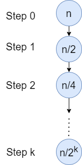
Let’s try to derive this time complexity for an input array of size n. At the beginning we have to search the target among n integers, so Search Space = n. Our goal is to find the number of steps it will take us to reach the target. Let this be k. Have a look at the diagram below to understand how the Search Space is changing at every step of the algorithm –

At step k indicates the step where we found our target, so search space = 1.

n/2^k =1, implies 2^k = n. Thus we have k = log2n.

Best Case Time Complexity – O(1), this happens if the middle element is our target and we get our answer in the very first step.

Worst and Average Case Complexity – O(log2n), as explained above.

Space Complexity

We are consuming constant space here, so space complexity is O(1).

Let’s have a look at some examples where we can use Binary Search.

Examples

Example 1: Guess Number Lower or Higher

Problem Statement

We are playing the Guess Game. The game is as follows:

I pick a number from 1 to n. You have to guess which number I picked.

Every time you guess wrong, I will tell you whether the number I picked is higher or lower than your guess.

You call a pre-defined API int guess(int num), which returns three possible results:

• -1: Your guess is higher than the number I picked (i.e. num > pick).
• 1: Your guess is lower than the number I picked (i.e. num < pick).
• 0: your guess is equal to the number I picked (i.e. num == pick).

Return the number that I picked.

Constraints:

• 1 <= n <= 231 - 1
• 1 <= pick <= n

Solution –

By looking at this problem, we can easily establish that it looks very similar to the basic logic of the Binary Search algorithm. With the given three conditions, we can easily construct the complete code. Have a look at it below –

Example 2: Search Insert Position

Problem Statement

Given a sorted array of distinct integers and a target value, return the index if the target is found. If not, return the index where it would be if it were inserted in order.

Constraints:

• 1 <= nums.length <= 104
• -104 <= nums[i] <= 104
• nums contains distinct values sorted in ascending order.
• -104 <= target <= 104

Solution –

The first fact to note is that the array nums is sorted and contains unique values. There are 2 parts to the question –

• If target is present, just return its index in nums, denoted by variable low.
• If its not present, then we need to return the index at which it can be inserted. In this case, we return the index of number just lower than target, also given by variable low.

So this means we can use Binary Search as-is and just return low as the result for both these cases. Let’s have a look at the code –

In further posts, we will have a look at the different variants of the main algorithm along with their templates, which can be used to solve many interesting problems. So stay tuned for more!