Google Kickstart Round A 2021: Checksum

In this post we’ll look at the Checksum problem from Google Kickstart Round A 2021 which may look confounding at first glance but interesting nonetheless.

Checksum – Problem Statement

Grace and Edsger are constructing a N×N boolean matrix A. The element in i-th row and j-th column is represented by A_i,j. They decide to note down the checksum (defined as bitwise XOR of given list of elements) along each row and column. Checksum of i-th row is represented as RiRi. Checksum of j-th column is represented as Cj.

For example, if N=2, A=[1101], then R=[10] and C=[01].

Once they finished the matrix, Edsger stores the matrix in his computer. However, due to a virus, some of the elements in matrix A are replaced with −1 in Edsger’s computer. Luckily, Edsger still remembers the checksum values. He would like to restore the matrix, and reaches out to Grace for help. After some investigation, it will take B_i,j hours for Grace to recover the original value of A_i,j from the disk. Given the final matrix A, cost matrix B, and checksums along each row (R) and column (C), can you help Grace decide on the minimum total number of hours needed in order to restore the original matrix A?

Input

The first line of the input gives the number of test cases, T. T test cases follow.

The first line of each test case contains a single integer N.

The next N lines each contain N integers representing the matrix A. j-th element on the i-th line represents Ai,j.

The next N lines each contain N integers representing the matrix B. j-th element on the i-th line represents Bi,j.

The next line contains N integers representing the checksum of the rows. i-th element represents Ri.

The next line contains N integers representing the checksum of the columns. j-th element represents Cj.

Output

For each test case, output one line containing Case #x: y, where x is the test case number (starting from 1) and y is the minimum number of hours to restore matrix A.

For all the limits and test cases you can check the official problem page for Checksum here.

Solution

First let’s take a simple test case and analyze how we can calculate the minimum hours to restore the original matrix. For N = 2, we are given following 2 matrices –

Logically the first thing we will do is to look at all the lost cells having -1. Choose the one with the least cost to restore and greedily restore the others in the same manner. We can repeat these steps until we each row and each column have either none or 1 more cell left to restore.

One thing to note is that after restoring each cell, say Aij, the total count of the cells to restore from i-th row and j-th column each gets decreased by 1. Next important thing is that, in anywhere in our calculation we don’t require either the Row Checksum matrix or the Column Checksum matrix. So the these inputs will be considered as trivial.

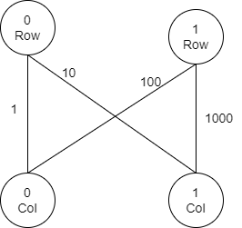
This gives an idea that we need to treat all the rows and columns independently. Then the complete problem can be modeled as a undirected graph with N row vertices and N column vertices, that is, 2N vertices. Each cell Aij can be thought of as an edge from i-th row to j-th column. The given testcase will now look like –

Arriving to this conclusion, we can now paint the complete picture. Our goal is to minimize the total cost/hours to restore the complete matrix. To achieve this goal, we need to select the edges with the minimum cost in a way which can help us to restore the rest of the edges. That is, we can separate the edges into two groups –

Group A: Edges which should be restored with some cost. We need to find the sum of the costs of all such edges.

Group B: Edges which can automatically restored without any cost using the restore edges of Group A and the checksum matrices.

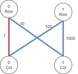
Let’s go back to our testcase and categorize all the edges –

First we will restore the cell A[0,0] with cost 1. Using this restored cell and the row checksum, we can easily restore A[0,1]. In the same manner A[1,0] and A[1,1] can also be restored without any cost. Thus the total hours to restore the complete matrix comes out to be 1.

If you will carefully look at these edges, you will find that they all belong to a cycle A[0,0]->A[1,0]->A[1,1]->A[0,1]. This means if we break this cycle by removing the edge with the minimum cost (A[0,0]) we can easily restore the rest of the edges that form the cycle.

Thus we found Atlantis… ! Just kidding 🙂

The brute force solution will entail traversing all the N² edges and running a DFS on each edge to remove the cycles. The total time complexity of this solution will then be N⁴. That’s quite huge, isn’t it?

Another way to solve it would be to first find the total weight of all the Group B edges. Then substract this from the total weight of the graph to finally get the cost of Group A edges which will be our final answer. Intuitively, Group B edges all come together to construct Maximum Spanning Tree. So we can either use Kruskal’s or Prim’s algorithm to get the cost of the Maximum Spanning Tree.

Kruskal’s Algorithm

Here, first we will generate the edge list for all the lost cells, where each item will be [Costij, i, j]. Then we will sort the edges in descending order of costs and traverse them one by one. If the edge belong to a cycle, we can safely ignore it. Otherwise, this edge will form the part of the MST.

For cycle detection, we can use Union Find algorithm. There are two flavors of Union find – Simple Union find having time complexity of O(N) & Union Find by Rank and Path Compression having time complexity of O(logN). We will be using the latter method –

Union Find by Rank and Path Compression –

#For Cycle Detection in MST
def find(x,parent):
    if parent[x] != x:
        parent[x] = find(parent[x],parent) # path compression - by changing the parent to the root of the subtree for all the nodes along the path 
    return parent[x]

def union(x, y,parent,rank):
    px, py = find(x,parent), find(y,parent) # find the parent nodes
    if px != py: # if parents are different, then do the merge
        if rank[px] < rank[py]: # Cosider the parent with the highest rank to be the super parent
            px, py = py, px
        parent[py] = px # Change the parent of the smaller rank subtree(Union Operation)
        rank[px] += rank[px] == rank[py] # Accordingly increase the rank of super parent tree, if the ranks of both px and py are same

Maximum Spanning Tree

To construct the graph, we will have 2N vertices, 0 To N-1 will be Row vertices and N to 2N-1 will be Column vertices.

def kruskal_solve(n,arr,cost):
    rest=0 #Total weight of Group B edges of MST
    parent=[0]*(2*n) 
    rank=[0]*(2*n)
    edges=[]
    total=0 #Total cost of all the edges
    for i in range(n):
        for j in range(n):
            if arr[i][j]==-1:
                total+=cost[i][j]
                edges.append([cost[i][j],i,j]) #construct edge matrix
                parent[i]=i #Intialize parent for Row Vertex
                parent[n+j]=n+j #Intialize parent for Column Vertex 
                
    edges.sort(reverse=True) #Sort edges in Descending Order
    for c,i,j in edges:
        #find the parents of the subtrees to which the nodes belong
        x=find(i,parent) 
        y=find(n+j,parent)
        if x!=y: #if the edge (i,j) is not part of a cycle
            rest+=c # increase the cost of MST by c
            union(i,n+j,parent,rank) #Add the edge to the MST
        
    return total-rest #Final Cost of Group A edges = Cost to restore orginal matrix

T = rri()
for t in range(1, T + 1):
    n = rri() #single input
    arr = []
    for i in range(n): #2D
        arr.append(rra())
    cost=[]
    for i in range(n): #2D
        cost.append(rra())
    rowc=rra() #Row and column checksums are trivial
    colc=rra()
    
    print('Case #{}: {}'.format(t, kruskal_solve(n, arr,cost)))

Time Complexity - O(N²logN)

Here it takes N²logN time to sort all the N² Edges. Then while traversing all the sorted edges, an extra logN time goes for cycle detection by Union Find Algorithm. So overall, Kruskal's algorithm costs O(N²logN) time.

Space Complexity - O(N²)

O(N²) space is used for storing the N² edges. Parent and Rank matrices each take up O(N) space. O(logN) space is used for sorting. So overall space complexity comes out to be O(N²)

Prim's Algorithm

We first generate an adjacency list for each of the 2N vertices by appending the connected vertex and edge cost to the list. The weights of all the vertices are set to -1 and they are all initially unvisited. The complete implementation can be found below -

def prim_solve(n,arr,cost):
    rest=0
    adj = collections.defaultdict(list)
    weight=[-1]*(2*n) #Intialize the weights of all vertices as -1
    visited=[0]*(2*n) #All the vertices are initially unmarked
    total=0 #Total cost of all the edges
    for i in range(n):
        for j in range(n):
            if arr[i][j]==-1:
                total+=cost[i][j]
                adj[i].append([cost[i][j],n+j]) #Generate Adjacency list
                adj[n+j].append([cost[i][j],i])
    if(adj.keys()): #Set the first vertex as the starting vertex of MST
        weight[list(adj.keys())[0]]=0

    for i in adj.keys(): #Traverse all the vertices of the Adjacency list
        max_vertex=-1
        for j in adj.keys(): #Calculate unvisited max_vertex having the highest weight
            if not visited[j] and (max_vertex==-1 or weight[j]>weight[max_vertex]):
                max_vertex=j
        visited[max_vertex]=1 #Mark it as visited
        if weight[max_vertex]!=-1: #Check if the max-vertex is not isolated
            rest+=weight[max_vertex] # increase the cost of MST by the weight of max_vertex
        for c,j in adj[max_vertex]: #Traverse the children nodes of max_vertex
            if not visited[j] and c>weight[j]: #Update the weights of unvisited children
                weight[j]=c
    return total - rest #Final Cost of Group A edges = Cost to restore orginal matrix

Time Complexity - O(N²)

It costs O(N²) time to loop through all the 2N vertices 2N times.

Space Complexity - O(N²) Same like Kruskal's implementation

For dense graphs, we can achieve better time complexity using Prim's algorithm as compared to Kruskal's algorithm.

If you have any questions or thoughts, let me know in the comments below. Until then, Happy coding!